Research Article

 

SVM Based Classification and Prediction System for Gastric Cancer Using Dominant Features of Saliva

 

Muhammad Aqeel Aslam 1, Cuili Xue 1, Kan Wang 1, Yunsheng Chen 1, Amin Zhang 1, Weidong Cai 2, Lijun Ma 3, Yuming Yang 1, Xiyang Sun 3, Manhua Liu 1, Yunxiang Pan 1, Muhammad Asif Munir 4,  Jie Song 1, Daxiang Cui 1, 3, 5

 

1 Institute of Nano Biomedicine and Engineering, Shanghai Engineering Research Centre for Intelligent Diagnosis and Treatment Instrument, Department of Instrument Science and Engineering, School of Electronic Information and Electrical Engineering, Yantai Information Technology Research Institute, Shanghai Jiao Tong University, 800 Dongchuan Road, Shanghai 200240, China.

2 School of Computer Science, Faculty of Engineering and IT, The University of Sydney, NSW 2006, Australia.

3 Department of Oncology, Shanghai Tongren Hospital, School of Medicine Shanghai Jiaotong University, Shanghai 200336, China.

4 Electrical Engineering Department, Swedish College of Engineering & Technology, Rahim Yar Khan, Punjab, Pakistan.

5 National Center for Translational Medicine, Collaborative Innovational Center for System Biology, Shanghai Jiao Tong University, 800 Dongchuan Road, Shanghai 200240, China.

 

* Corresponding author. E-mail: dxcui@sjtu.edu.cn

 

Received: Jul. 25, 2019; Accepted: Dec. 26, 2019; Published: Dec. 26, 2019

 

Citation: Muhammad Aqeel Aslam, Cuili Xue, Kan Wang, Yunsheng Chen, Amin Zhang, Weidong Cai, Lijun Ma, Yuming Yang, Xiyang Sun,  Manhua Liu, Yunxiang Pan, Muhammad Asif Munir,  Jie Song, and Daxiang Cui, SVM Based Classification and Prediction System for Gastric Cancer Using Dominant Features of Saliva. Nano Biomed. Eng., 2020, 12(1): 1-13.

DOI: 10.5101/nbe.v12i1.p1-13.

 

Abstract

Machine learning techniques are widely used for the diagnosis of cancers. In this study, we proposed a classification and prediction system for the diagnosis of gastric cancer based on saliva samples. Gastric cancer (GC) is classified into early gastric cancer (EGC) and advanced gastric cancer (AGC). The diagnosis of GC at an early stage will improve the survival rate. Computer-aided diagnostic (CAD) systems can assist the radiologists in the diagnosis of EGC. 220 saliva samples were collected from the non-cancerous and gastric cancerous persons and analyzed using high-performance liquid chromatography-mass spectrometry (HPLC-MS). Fourteen amino acid biomarkers were sufficient to distinguish the persons from malignant to benign and were observed in the saliva samples with dominant peaks. We used the support vector machine (SVM) for binary classification. The processed Raman dataset was used to train and test the developed model. SVM based neural networks were established using different kernels, which produced different results. Accuracy, specificity, sensitivity, and receiver operating characteristics (ROC) were used to evaluate the proposed classification model, along with mean average error (MAE), mean square Error (MSE), sum average error (SAE), and sum square error (SSE). We achieved an overall accuracy of 97.18%, specificity of 97.44%, and sensitivity of 96.88% for the proposed method. This established method owns the prospect of clinical translation.

 

Keywords: Machine learning; Gastric cancer classification; Support vector machine; Accuracy; Dominant peaks; Specificity; Sensitivity; ROC

 

Introduction

Gastric cancer (GC) is the fourth commonest cancer in the world and the second leading cause of cancer-associated deaths in China [1, 2].  GC is classified into two stages, which are early gastric cancer (EGC) and advanced gastric cancer (AGC), stages I and II belong to EGC, and stages III and IV belong to AGC [3]. The early diagnosis of GC is very crucial for increasing the survival rate because GC is a very aggressive type of cancer [4, 5]. If GC is diagnosed in an early stage, the survival rate is very high up to 62.8%, whereas at AGC, the survival rate is very low, up to 24% [6]. Only Japan has a five-year survival rate of more than 90%, which is possible only due to the early screening of the patients [7]. In Europe, the five-year survival rate is 20 to 30% only [8]. In recent years, tumor-associated antigens and biomarkers have analyzed for the prognosis of the cancer disease. These antigens or biomarkers can be found in the urine, blood, saliva, or breath of the human [9]. Cancer cells do not behave like normal cells and cause a change in the human body. This change rate depends on the stage of cancer, along with the location of the cancer cells. GC is associated with several factors, which include living standards, living environment, lifestyle, and genetic factors [10].  Quite a lot of studies have been stated in the literature and are based on diverse approaches that could permit premature cancer investigation and prediction [11-14]. Explicitly, these studies described methods associated with the profiling of circulating miRNAs that have established as promising biomarkers for cancer detection and identification. However, these methods suffer from low sensitivity concerning their usage in screening at early phases and differentiating amongst benign and malignant tumors. Several features regarding the forecasting of cancer outcomes based on gene expression signatures are discussed by Koscielny [15] and Michiels et al. [16]. The biopsy and endoscopy are widely used methods for the diagnosis of cancer in clinics. These methods are invasive and require expensive equipments, professional skills, and a long procedure for the diagnosis of cancer [17]. Moreover, these methods are not efficient enough to diagnose EGC due to vague symptoms [18]. The mortality rate may increase due to the delayed diagnosis and inadequacies of the staging system [19, 20]. In the last few years, researchers have developed non-invasive methods for the screening of EGC patients. VOC, miRNA, and sera biomarker-based prognosis methods have been developed. Recently, blood biomarker tests and salivary diagnostics methods have been developed to overcome these challenges [21]. Saliva behaves like a mirror of health, and it can be collected accurately without any medical consideration [22]. Moreover, saliva diagnostics methods are non-invasive, efficient and require little time to diagnose GC. To solve the key problems of early gastric cancer diagnosis, our team firstly proposed the strategy to establish the gastric cancer pre-warning and early diagnosis system in 1998 [23]. It consists of three parts, early gastric cancer diagnosis chips, gastric cancer pre-warning database, and the information processing system. With the development of nanotechnology, the emerging nanotechnology brings new chances to solve the key scientific problems of early warning and early diagnosis of gastric cancer [24-26]. The application of computer-aided diagnostic (CAD) systems has reduced the misclassification rate in cancer diagnosis and improve the time efficiency in data analysis. Artificial intelligence (AI) is playing an important role in every aspect of daily life for the last few decades. Recently, it has gained the attention of the researchers, especially in the field of aviation, medicine, robotics, and industrial applications. Machine learning (ML) techniques as the way to realize AI, includes two types, (i) Supervised ML (ii) Unsupervised ML ML consists of four stages, input data collecting, model selecting, model training and model testing [27]. Researchers use ML to predicts the sequence of genes, which are responsible for the cancer generation cells [28, 29]. ML can also be employed to determine the prognosis and can improve the accuracy of cancer prediction [30]. A good model provides a high positive rate and high negative rate [31]. Support vector machine (SVM) was proposed by Vapink in 1995 [32]. This method has been used for classification, regression, structural risk minimization and density estimation [33, 34]. SVM is a powerful tool for pattern recognition tasks and does not explicitly depend on the dimensionality of the input data [35]. SVM was used to analyze gene expression to diagnose prostate cancer in the early stage, and to select gene and classification of the genes [36-38]. A variety of methods for baseline correction has studied for Raman spectra [39]. These methods include polynomial baseline correction [40], simulation-based methods [41, 42], and penalized least squares [43, 44]. In this work, we used SVM classifier to analyze the Raman data of amino acids from saliva samples to distinguish gastric cancer patients from healthy persons. Kernel trick was used in the proposed SVM system to achieve the possible higher accuracy. Finally, we extracted fourteen dominant Raman peaks and established the model, achieved an overall accuracy of 97.18%, specificity of 97.44%, and sensitivity of 96.88% for the developed model. This established method owns the prospect of clinical translation.

 

Experimental

Collection of the saliva samples

The study was conducted according to the Reporting Recommendations for Tumor Marker Prognostic Studies (REMARK) guidelines. All the saliva samples were collected from Shanghai Tongren Hospital. Informed consent was obtained from patients in accordance with the guidelines for the conduction of clinical research. All investigational protocols were approved by their Institutional Review Boards. When collecting the GC samples, three criteria were followed: (1) Clinical diagnosis of GC; (2) Excluding the patients with other malignancies; (3) Excluding the patients with metabolic diseases, mainly including diabetes. 220 volunteers, including 20 EGC patients, 84 AGC patients, and 116 healthy persons, provided the first saliva samples as a training set. The GC stage information was followed by the AJCC Cancer Staging Manual. The age and sex distribution were not important differences among EGC patients, AGC patients, and healthy persons, and it would lead the results without bias. Before collecting the saliva samples, the volunteers were required to clean the mouth and had refrained from eating and drinking for over 1 h. 4 mL of saliva sample was collected and centrifuged for 30 min at 12,000 rpm at 4 oC. Then, 2 mL of the supernatant was transferred into centrifuge tubes and stored at −70 oC. Table 1 shows the basic information and clinical characteristics of the volunteers. The following individuals were already gone through the screening for the GC using different techniques. We used this dataset for the preparation of the model. This classifier will help us in the prognosis of the new unseen data.

 

Table 1 The clinical characteristics of volunteers

Group	Number	Age (years)	Gender (M:F)
EGC	20	60 ± 8.6	13 : 7
AGC	84	53 ± 9	50 : 34
Controls	116	35 ± 10	67 : 49

 

Data pre-processing

Data processing was the key part of this study. Raman spectroscopy does not work on the principle of the absorption of the light, but it uses the scattering principle of the light, for the detection of the biomarker. Each data sample is characterized by some biomarkers, which were called features. The following steps were performed in the data processing phase before applying the ML method. After gathering the data from SERS, data processing was done. The first step of data processing was the baseline correction of the raw data. If the baseline does not correct properly, it may produce errors, which are leftover background and overfitting. A baseline should not cut into Raman band signal strength. The fourth order polynomial shown in the following equation was used for baseline correction.

.

(1)

After correcting the baseline, the noise was removed from the Raman spectrum. Without this step, the ML algorithm may produce errors in the diagnosis of the GC. The predicted model will misclassify the new data, so we cannot achieve the system’s stability or the system’s repeatability, which is necessary for neural networks. The Raman spectrum was affected by the five different types of noises, which include the 1/f noise component, dark current noise, readout noise, background fluctuations, and the noise produced by the photon due to the uncertainty. Noise is the unwanted signal that degrades the information of the actual data.   For smoothing and noise removal from the Raman spectrum, we tried different filters, which include first-order derivative filter, second-order derivative filter, median filter, moving average filter, and Savitzky-Golay filter. We achieved better results from the Savitzky-Golay filter, as it smooths the data much better than other filters, and the band shape is also preserved better. Whereas, the median filter and moving average filters tend to shift the band, which is again adding the disturbance in the original signal, which may lead to introduce an error in the Raman spectrum. Therefore, we used a second-order Savitgzky-Golay filter to smooth the data. The equation for the second-order Savitgzky-Golay filter is given below.

) / (⧍λ^2).

(2)

Here, λ is the wavelength number, and y represents the spectral intensity.

 

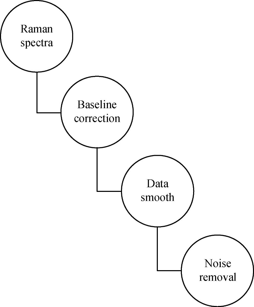
Fig. 1 Block diagram of data preprocessing, Preprocessing includes baseline correction, data smooth and noise removal from the saliva sample.

 

Features extraction

The following figure shows the Raman spectrum of the saliva sample. In this sample, there are more than three thousand data points. To make accurate, and precise prognostic for gastric cancer classification, a statistical analysis of the area under these fourteen peaks was carried out by using Labspec5. We selected fourteen Raman spectrum bands which showed significant difference between different groups and they were associated with fourteen amino acid biomarkers. These bands and their corresponding amino acids are shown in Table 2. The information of different organic compounds is detected at different locations of the bands. 

 

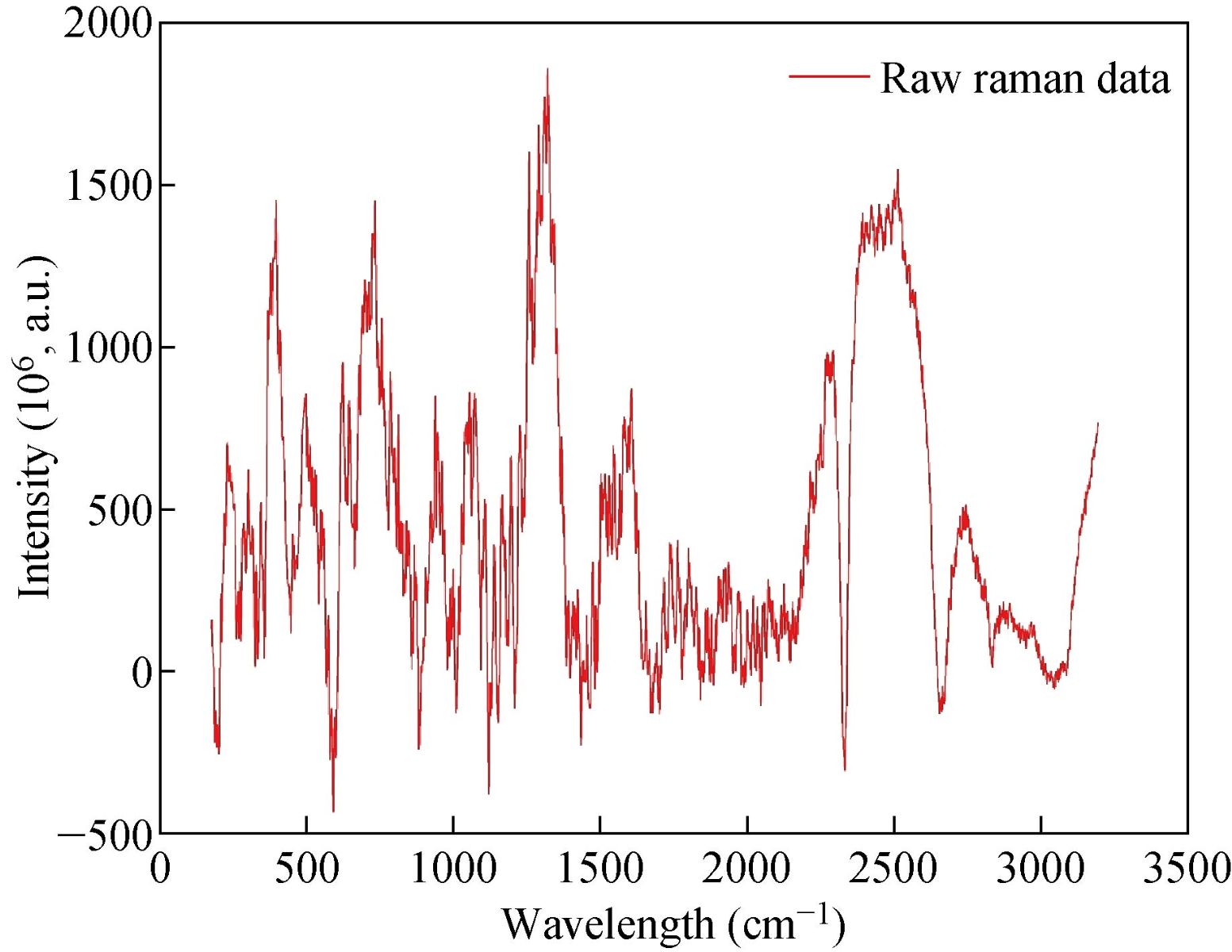
Fig. 2 Raman spectrum of input data.

 

Table 2  The relation between the fourteen bands as fingerprints and corresponding biomarkers

Band No.	Band position (cm−1)	Biomarkersa	Band No.	Band position (cm−1)	Biomarkersa
1	435	Gln, Hyl, Pro, Tyr	8	961	His, Glu, Pro, Tyr
2	488	Tau, Gly, EtN, Hyl, Tyr	9	1037	Tau, EtN, Ala, Pro, Tyr
3	530	Tau, Gln, His, Ala, Glu	10	1053	Tau, Gln, EtN, Hyl
4	642	His, Ala, Pro, Tyr	11	1109	Tau, Gln, EtN, His, Ala
5	725	Tau, Gln, His, Glu	12	1197	His, Hyl, Pro, Tyr
6	781	Gln, Glu, Pro, Tyr	13	1222	Hyl, Pro, Tyr
7	843	Tau, EtN, His, Ala, Hyl, Pro, Tyr	14	1450	Tau, Gly Gln EtN, Ala, Glu, Hyl, Pro

 

Classification methodology

Support vector machine has been extensively used for classification, regression, and density estimation. In SVM, the first step is to find the hyperplane. A line that separates two different classes is called a hyperplane.

(3)

The hyperplane separates all the data points belongs to the class xi by the following decision rule,

(4)

SVM chooses the separating hyperplane using the above equation. It calculates the maximal margin from the data points xi. The hyperplane should be far away from the data points, so when we classify new data to make true decisions. A separating hyperplane for the two-dimensional training set is shown in Fig. 3. Each pattern consists of a pair {xi,yi}. Let xi be a vector, and xi Rn and the corresponding labels be yi {-1,1}. The following equation was used to find the classifier using the SVM approach,

(5)

Here, ɑi are positive real constants, and b is real constant. In general, K(xi,x) represents the inner product operation and . We used linear hyperplane to separate data in the high dimensional space.

Fig. 4 shows the architecture of SVM with the kernel function. In Fig. 4, {-1,1} are the responses of the classifier, b is the real constant and K(x1,x2) = ϕ(x1),ϕ(x2) is called kernel function. We used the supervised machine learning technique for distinguishing the data from cancerous to non-cancerous data. We had the labeled data, which was used to train the model and estimate the desired output. We developed SVM based model which used for binary classification problem. The dataset was fed as an input to the classifier. We developed SVM based classifier, which is a discriminative classifier, belongs to the supervised machine learning technique. SVM classifies the data with the help of separating hyperplane. The hyperplane has divided the data into two classes, and each class lay on either side. We developed the SVM model using different kernels, including linear kernel, polynomial kernel, radial kernel, and sigmoid kernel. The kernel trick has enabled us to get the maximum accuracy of our particular model. Like any other ML model. Our proposed SVM model also consists of two phases, which are the training phase and the testing phase. The training phase is used to train the model from the labeled data, and once the model is trained, we used the developed model to check the performance of the developed model. If there is a large number of misclassification, it shows that the developed model needs to be improved by adjusting some parameters and get the maximum result, which is no or low misclassification. We used SVM with a linear kernel, whose decision boundary is a straight line. The equation of the SVM using a linear kernel is given below,

.

(6)

A network that uses RBF as an activation function is called the RBF network.  In radial basis function (RBF) based model, the output of the network depends upon the linear combination of radial basis function of the inputs and neuron parameters. The equation of the RBF kernel-based SVM is given below,

,

(7)

where x and x’ are the two data points, and |x-x|2 is the squared Euclidean distance between these two data points. In the RBF kernel-based model, two factors affect the performance of the developed model. These two factors are c and gamma. The gamma factor is used for the decision region. If the gamma value is low, we get the low decision boundary, whereas the decision region is very broad. If the gamma is high, the decision boundary is also high, with the decision boundaries around data points. Factor c is the penalty of misclassifying the data point. We need to keep c small for the good results of the SVM classifier. If the value of c becomes high, it will lead to high misclassification. Therefore, it is very necessary to keep the value of c small, so it does not have high bias and low variance. The equation of the SVM model using the polynomial kernel is shown below,

.

(8)

The equation of the SVM model using the sigmoid kernel is given below.

.

(9)

Here are kernel parameters. The performance of the SVM model depends upon these parameters. We used the kernel trick to get the maximum accuracy for each model. In GC based medical applications, a large amount of data is required for precise classification during the training phase. This constraint is hard to meet in practice for clinical data. In our work, we solved this issue by using the concept of fixed size saliva samples. The flowchart of the proposed model is shown in Fig. 5.

 

Algorithm 1 Our proposed SVM model for gastric cancer classification

Input : X = {x1,………….,xN}, x  X

Class label : Y = {Y1,Y2}, y Y

Initialize weights Parameters (w,ɑ,b,K)

Classifier: f(x) = w.ϕ(x) + b, xi = ϕ(xi)

Functional margin : yi(wTxi + b)

Distance to separator : r = y(wTx +b) / ||w||

Optimization kernel Function : f(x) =

RBF-kernel : f(x) =

Outcome: f(x) ≥1, if yi = 1

f(x)≤1, if yi = -1

 

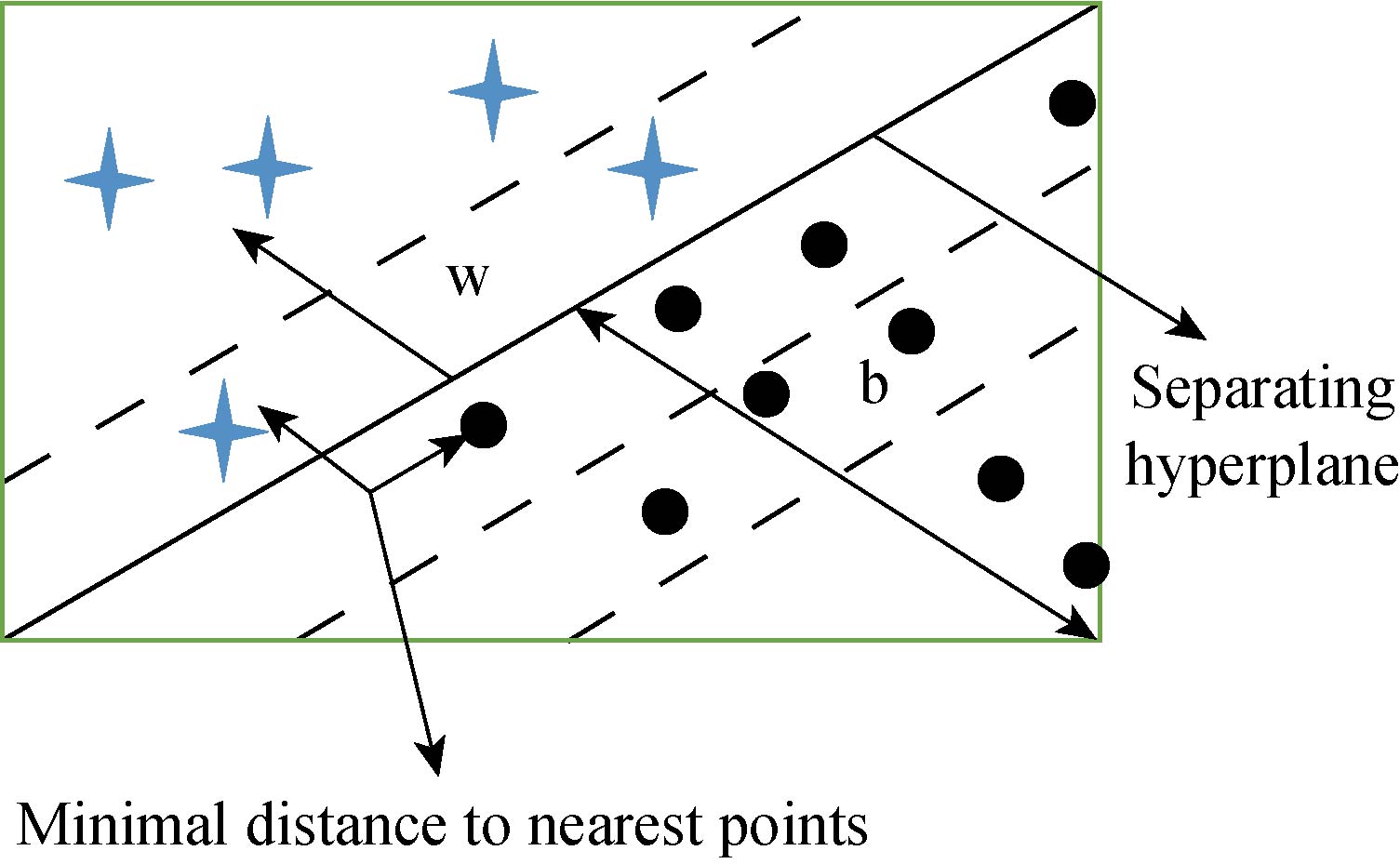
Fig. 3 Two dimensional training dataset for SVM.

 

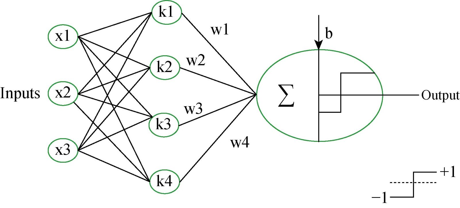
Fig. 4 Support vector machine architecture for binary classification.

 

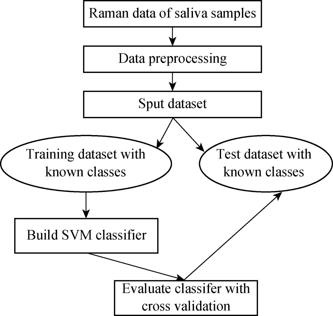
Fig. 5 Methodology of gastric cancer diagnosis model using SVM.

 

Performance evaluation

True positive (TP): When the person is healthy, and the neural network also recognizes it as healthy. True negative (TN):  When the person is a cancer patient, and the neural network also calculates it as a cancer patient. False positive (FP): When a person was labeled a cancer patient, but the neural network classifies it as a healthy person. False negative (FN): When a person was labeled a healthy person, but the neural network predicts as a cancer patient. True positive is also known as sensitivity, which is the ability of the classifier to identify the disease correctly. The true negative rate also called specificity. Specificity is the ability of the classifier to identify those who do not possess the disease. TN rate or specificity is a measure of the classifier to detect cancer patients.  Selectivity is the ability of the classifier to reject the false detection of a healthy person. The detection rate is defined as an average of sensitivity and specificity. These parameters were calculated as follows,

,	(10)
,	(11)
, and	(12)
.	(13)

The Raman data was divided into two parts, which are training data and test data. Training data consists of 70% of the total data, and test data consists of 30% of the total data.

 

Results and Discussion

Data processing

A high-quality saliva sample was required to produce an accurate diagnosis of GC. Saliva samples were obtained from SERS. A dataset was prepared by using saliva samples. This dataset was used for the training phase and the testing phase. The saliva samples were processed, and then we used these samples as an input to the classifier. The saliva samples were two dimesnsional data. On the x-axis, we have the wavelength number, whereas, on the y-axis, we have the intensity in 10-6 a.m.u. The following figure shows the Raman spectrum before and after the baseline Figure 6 shows that the baseline of the Raman spectrum has shifted. Moreover, there is no negative value in the Raman spectra. After performing the baseline correction, we removed the noise from the Raman spectrum. Fig. 7 shows the result of the second-order Savitzky-Golay filter for smoothing and removing the noise from the Raman data.

 

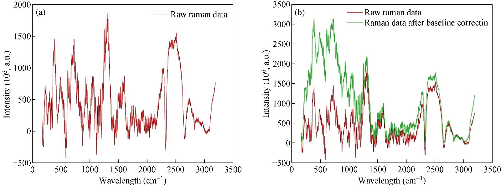
Fig. 6 Results of baseline correction on Raman spectrum.

 

 

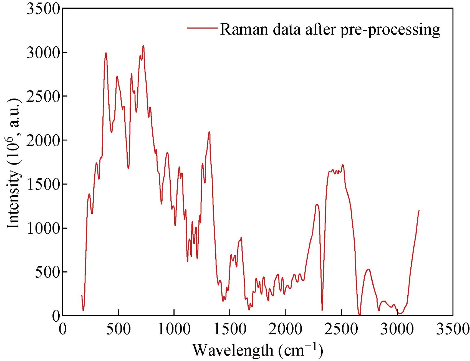
Fig. 7 Raman spectrum after data preprocessing.

 

Performance analysis of SVM classifier

We developed the classification model using the SVM technique. In the development of the model, training and generalization errors were produced. Errors on the training data called misclassification, whereas the error on the testing data is called the generalization error. Our proposed classifier model fits the training data well and predicted the testing data accurately. We closely observed the test error rate and the training error rate to avoid the model overfitting phenomenon. After the development of the classification model by using the proposed technique, we estimated the performance of the developed classifier. The performance of the proposed classifier was measured in terms of accuracy, selectivity, specificity, and detection rate. These parameters were used to establish the overall performance of the classifier. In our study, we have two outputs, that is either the person is healthy, or the person is cancer patients. The performance of the classifier was estimated using 10-fold cross-validation. To avoid the overfitting issue, we used an ES approach. We controlled the error of the network during the training phase and stopped the training if the model undergoes the overfitting. The accuracy of the SVM with a linear kernel was low, and it was nearly 65%, and the misclassification ratio was also very high. Therefore, SVM with linear kernel did not use in this study. We developed SVM based model with RBF kernel. Fig. 8 shows the results of the SVM based models in terms of confusion matrices. There were seventy-one instances used in the test data, thirty-nine out of them were malignant, and thirty-two were benign. In linear SVM, thirty-one benign cases were correctly predicted by the model. Whereas, for the malignant cases, thirty-nine cases, and our model predicted thirty-four cases correctly. This model misclassified six samples. In Radial kernel-based SVM, out of seventy-one, six cases were misclassified, out of these six, four of them were from the malignant class and remaining two from the benign class.  In polynomial kernel-based SVM, six cases were misclassified by the model in the malignant class, and five cases were misclassified in the benign class. In sigmoid kernel-based SVM, there were fourteen instances, which were not predicted correctly, out of these fourteen, nine instances were from the benign class, and the five were from the malignant class. The result of test data is shown in Fig. 8 for the linear based kernel SVM model, radial based kernel SVM model, polynomial based kernel SVM model, and sigmoid based kernel SVM model. Table 3 shows the parameters and properties of each model produced during this study. Table 4 shows the comparison of different models, which were developed during this work. The maximum accuracy was achieved by linear kernel-based SVM with 92.96% accuracy. The polynomial kernel-based SVM model produced the minimum accuracy.  The performance of the polynomial kernel-based SVM model was lowest, whereas the sigmoid kernel-based SVM model has achieved better accuracy.  Therefore, we optimized our model to get higher accuracy. These developed models have shown low accuracy. Therefore, we optimized the radial based kernel SVM model to achieve higher accuracy. The result of the proposed optimized model is shown in Fig. 9. Out of seventy-one instances, which were used to test the performance of the proposed optimized model. There were only two instances that were misclassified by the optimized model. Out of these two instances, one instance was misclassified in benign class, and the other instance was misclassified in the malignant class. This model gives us an accuracy of 97.13%, which is very high, and we can use this model to predict the new data. We used epsilon value and cost function to optimize the model. These parameters are called hyper-parameter optimization. It helped us in selecting the best model. The cost value played an important role in the selection of the best model for this study. We select the cost function in such a way that if it goes beyond a certain value, it will end up with under-fitting. The default value of the cost function is 1, and if the value of the cost function goes above the selected value, it will lead to a high penalty for non-separable points, which would result in a higher number of support vectors. In the case of higher the number of support vectors, the model would become overfitting. The performance of that model decreases, and they do not produce high accuracy results. Therefore, we considered optimal cost function value to achieve high accuracy, high specificity, high sensitivity, and high detection rate. Since we used this model for the prediction of new data, so the model should have a high accuracy rate.  First, we used a large range of epsilon value and cost function. After the analysis of the following figure, we conclude that we can reduce the value of the cost function.  On the x-axis, we have the epsilon value, which ranges from 0 to 1, with an increment of 0.1, and on the y-axis, we have the cost value, which ranges from 2(2:9).  We have eleven different epsilon values along with eight different values of cost. It provides us eighty-eight different combinations. The epsilon value affects the number of support vectors. The complexity and generalization capability of the network depend on the epsilon value. The epsilon value determines the level of accuracy of the approximated function. If the epsilon value is larger than the range of the target, we cannot achieve good accuracy. We have used a 10-fold cross-validation method for the sampling method. The best model was obtained at a cost function value of 16 with an epsilon value of 0.2. Cross-validation is a technique to evaluate the performance of the model. In 10-fold cross-validation, the original data is partitioned randomly into ten equal sizes of subsamples, a single subsample was retained as validation data, and nine subsamples were used as training data. The cross-validation process was repeated ten times, with each of the ten subsamples used exactly once as the validation data. The ten results from the folds were averaged to produce a single estimation. These values selected in such a way that to get the optimal solution. From Fig. 10, we can conclude that the dark region is representing the less misclassification error, it is also telling us that here we have a low value of cost function with different values of epsilon. Table 5 shows the results of the parameters used in the optimized model. These parameters include the SVM type, SVM kernel, cost value, gamma, number of support vectors, number of classes, and number of vectors in each class. The results of the optimized model are shown in Table 6. The performance parameters include accuracy, specificity, sensitivity, selectivity, and detection rate for the optimized model. Area under curve (AUC) was also calculated for the developed models to evaluate the performance of the classifier. From Fig. 11, we can conclude that the greater the AUC better is the performance of the model. AUC was used in this study to determine which model predicts the classes with much more accuracy. We had developed four different models, AUC of the four models are shown in Fig. 11. Here, the true positive rates plotted against the false-positive rates. ROC tells us how much our developed is capable of distinguishing between classes. ROC is a probability curve. In our study, we have two classes, one is a positive class (patients), and the second is a negative class (healthy). AUC is the most important metric for the evaluation of the classifier. For 100% accuracy, these two curves must have to be separable, or there is no overlap. It means that an ideal model had able to distinguish the negative class and positive class perfectly. We optimized the radial kernel-based SVM model by using epsilon value and cost function to achieve higher accuracy among all the developed models. The AUC of the proposed optimized method has shown in Fig. 12, which indicates that the developed model has accurately distinguished between the patients and the healthy persons. Fig. 12 also indicates that the model is neither in under-fitting nor in over-fitting conditions. After optimizing the model, the number of misclassification instances has reduced to a large extent, making the system more reliable and accurate.

 

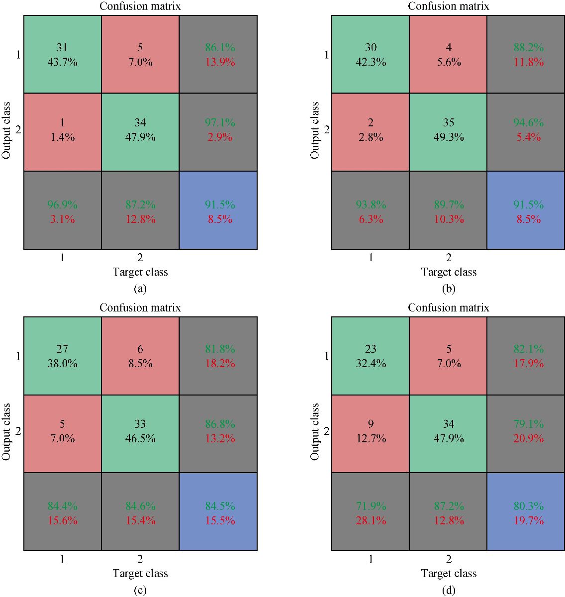
Fig. 8 Confusion matrices of SVM based neural netowrks wirh different kernels: (a) Linear kernel; (b) Radial kernel; (c) Polynomial kernel; and (d) Sigmoid kernel.

 

Table 3 Properties of the different SVM models using different kernels

Parameters	Properties of the radial based model	Properties of linear based model	Properties of polynomial based model	Properties of sigmoid based model
SVM – type	C- Classification	C – Classification	C – Classification	C – Classification
SVM- kernel	Radial	Linear	Polynomial	Sigmoid
Cost function	1	1	1 (3rd-degree polynomial)	1
Gamma	0.07142857	0.07142857	0.07142857	0.07142857
Number of support vectors	54	30	54	44
Number of classes	2	2	2	2
Class B (benign)	29	16	26	22
Class M (malignant)	24	14	28	22

 

Table 4 Performance parameters of the SVM models

Performance parameters	Radial model	Linear model	Polynomial model	Sigmoid model
Accuracy	0.8873	0.9296	0.7324	0.7887
Kappa Value	0.7685	0.8574	0.4291	0.5672
Sensitivity	0.9744	0.9487	1.0000	0.8718
Specificity	0.7812	0.9062	0.4062	0.6875
Detection Rate	0.8778	0.9274	0.7031	0.7796

 

 

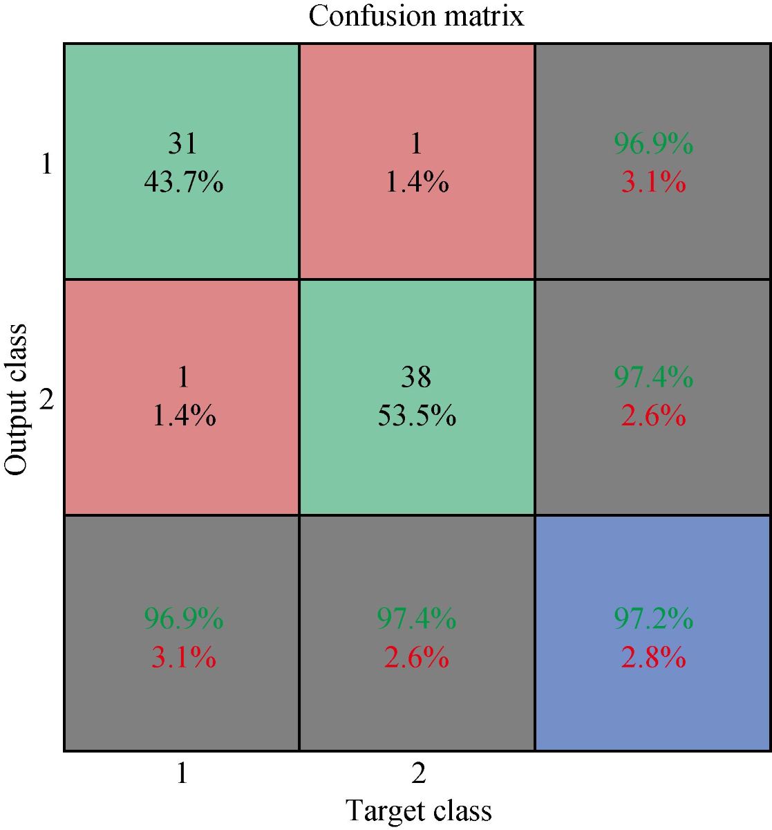
Fig. 9 Result of proposed optimized model.

 

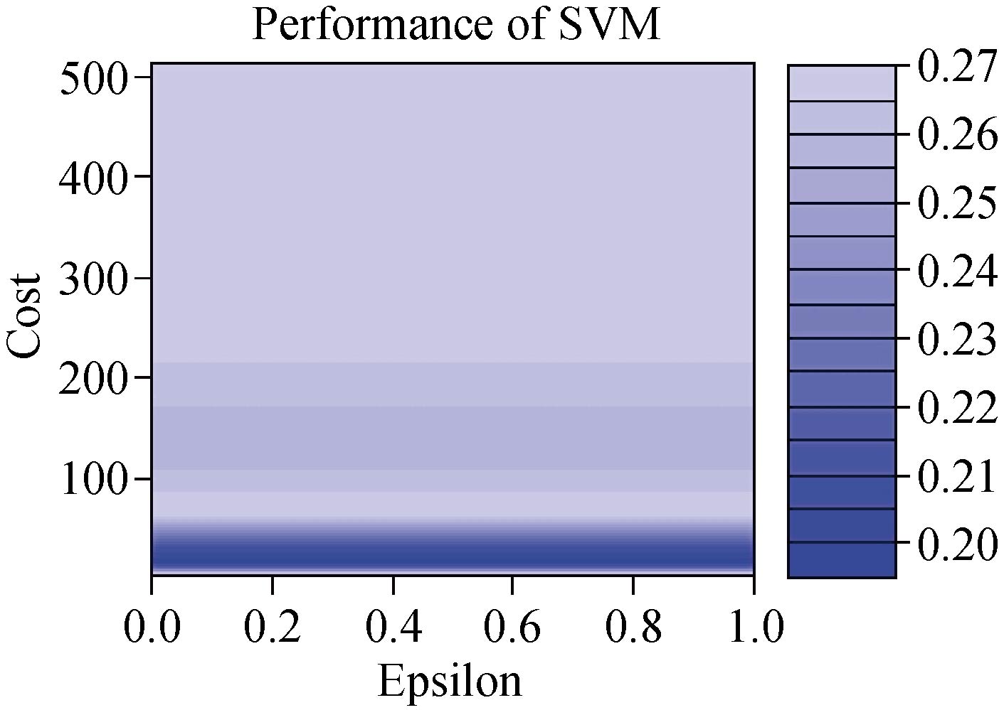
Fig. 10 Performance of optimized SVM classifier.

 

Table 5 Properties of optimized SVM model

Parameters of optimized model	Properties of optimized model
SVM – type	C – Classification
SVM – kernel	Radial
Cost function	16
Gamma	0.07142857
No. of support vectors	43
Number of classes	2
Number of support vectors in Class B	23
Number of support vector in Class M	20

 

Table 6 Performance parameters of the optimized proposed SVM model

Performance parameters	Results of optimized model
Accuracy	0.9718
Kappa value	0.9431
Specificity	0.9744
Sensitivity	0.9688
Detection rate	0.9716

 

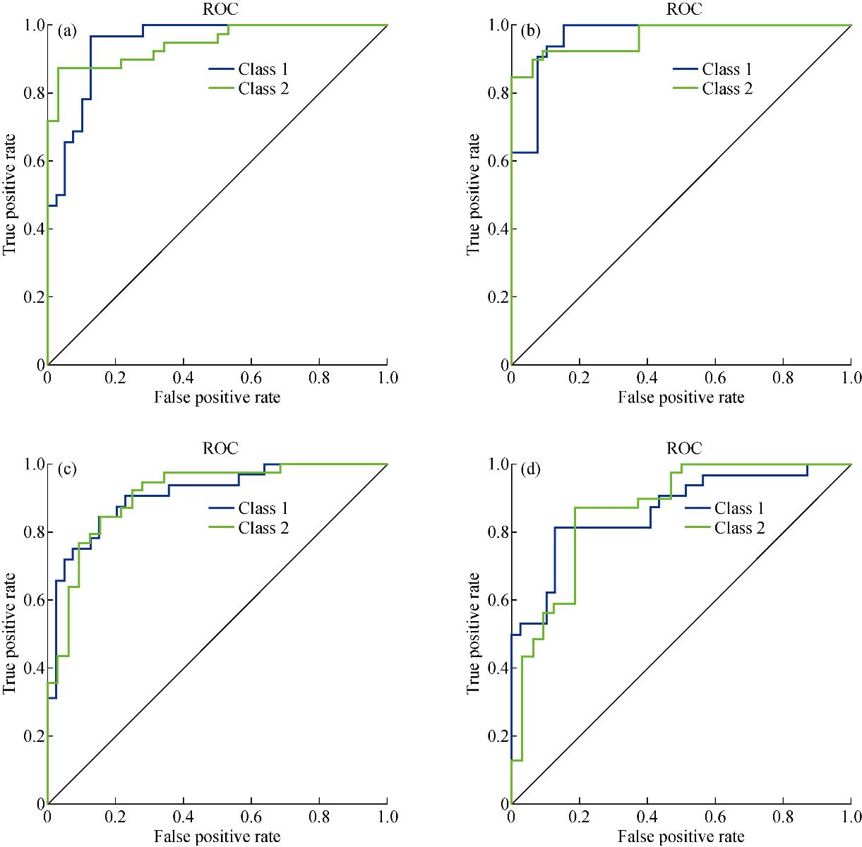
Fig. 11 Recover operating characteristics curve: (a) Liner SVM; (b) Radial SVM; (c) Polynomial SVM; and (d) Sigmoid SVM.

 

 

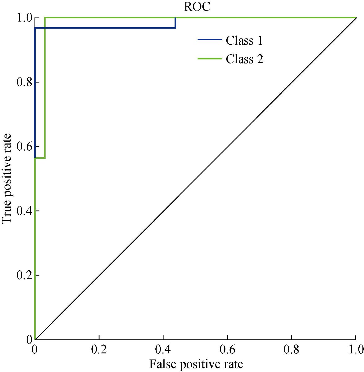
Fig. 12 ROC for proposed classification model.

 

Conclusions

In summary, fourteen amino acids as biomarkers were identified in human saliva. These fourteen biomarkers were used to distinguish GC patients from healthy persons. The saliva Raman dataset was collected by using SERS sensors. After getting the data, it was processed by data processing techniques, which include the removing of spikes, smoothing the raw data, and correcting the baseline. After these steps, we extracted the dominant peaks from the saliva samples. The dominant peaks were fed into the SVM classifier for the classification of the Raman data. We classify the saliva samples by using the SVM technique. SVM based classifier was used with different kernels to get the maximum efficiency and accuracy by using kernel trick. Each kernel produced a different outcome. Based on the achieved results, the sigmoid kernel has produced the best classification results with an accuracy of 97.18% %, specificity of 97.44%, and specificity of 96.88% during the testing phase, whereas the results of the other kernel-based models, SVM has not produced good results. Our proposed method for the classification of GC is non-invasive, cheap, and faster. With the combination of SERS based sensors, our proposed model has provided us an entirely new diagnostic way of GC. The proposed model is capable of playing an important role in clinics. The target and challenge of this study were to build a classifier for gastric cancer from saliva samples. The proposed model is precise and reliable.  The overall performance of the proposed system is very high.

 

Acknowledgements

This work was supported by 973 Project (2017FYA 0205304), National Natural Science Foundation of China (No. 81225010, 81028009 and 31170961), and the Research Fund of Yantai Information Technology Research Institute of Shanghai Jiao Tong University. The discussion with Prof. Mark I. Ogden in the Department of Chemistry of Curtin University is also gratefully acknowledged.

 

Conflict of Interests

The authors declare no competing financial interests.

 

References

1.       L.A. Torre, F. Bray, R.L. Siegel, et al., Global cancer statistics, 2012. CA Cancer J. Clin, 2015, 65(2): 87-108.

2.      Y. Li, X. Li, X. Xie, et al., Deep learning based gastric cancer identification. Proceedings of the 2018 IEEE 15th International Symposium on Biomedical Imaging (ISBI 2018). Washington, DC, USA, Apr. 4-7, 2018: 182–185. 

3.     Y. Chen, Y. Zhang, F. Pan, et al., Breath analysis based on surface-enhanced raman scattering sensors distinguishes early and advanced gastric cancer patients from healthy persons. ACS Nano, 2016, 10: 8169-8179.

4.      D.A. Daniel, K.Thangavel, Breathomics for gastric cancer classification using back-propagation neural network. Journal of Medical Signals and Sensors, 2016,  6(3): 172-182.

5.     Y. Zheng, K. Wang, J. Zhang, et al., Simultaneous quantitative detection of helicobacter pylori based on a rapid and sensitive testing platform using quantum dots-labeled immunochromatiographic test strips. Nanoscale Research Letters, 2016, 11: 62.

6.       S.R. Alberts, A. Cervantes, and C.J. Van de Velde, Gastric cancer : Epidemiology, pathology and treatment. Ann Oncol., 2003, 14(1): 31-36.

7.       M. Stock, F. Otto, Gene deregulation in gastric cancer. Gene, 2005, 360(1): 1-19.

8.       D.M. Parkin, F. Bray, J. Ferlay, et al., Global cancer statistics, 2002. CA Cancer J Clin, 2005, 55(2): 74-108.

9.      A. Hirayama, K. Kami, M. Sugimoto, et al., Quantitative metabolome profiling of colon and stomach cancer microenvironment by capillary electrophoresis time-of-flight mass spectrometry. Cancer Res, 2009, 69(11): 4918-4925.

10.   R. Wadhwa, S. Song, J.S. Lee, et al., Gastric cancer - Molecular and clinical dimensions. Nature Reviews Clinical Oncology, 2013, 10(11): 643-655.

11.   O. Fortunato, M. Boeri, C. Verri, et al., Assessment of circulating microRNAs in plasma of lung cancer patients. Molecules, 2014, 19(3): 3038-3054.

12.   H.M. Heneghan, N. Miller, and N,M.J. Kerin, MiRNAs as biomarkers and therapeutic targets in cancer. Curr Opin Pharmacol, 2010, 10(5): 543-550.

13.   D. Madhavan, K. Cuk, B. Burwinkel, et al., Cancer diagnosis and prognosis decoded by blood-based circulating microRNA signatures. Front Genet, 2013, 4(116).

14.   K. Zen, C.Y. Zhang, CirculatingmicroRNAs: A novel class of biomarkers to diagnose and monitor human cancers. Med Res Rev, 2012, 32(2): 326-348.

15.   S. Koscielny, Why most gene expression signatures of tumors have not been useful in the clinic. Sci Transl Med, 2010, 2(14): 14ps2. 

16.   S. Michiels, S. Koscielny, and C. Hill, Prediction of cancer outcome with microarrays: A multiple random validation strategy. Lancet, 2005, 365(9458): 488-492.

17.   K.H. Kim, S.A. Jahan, and E. Kabir, A review of breath analysis for diagnosis of human health. Trends in Analytical Chemistry, 2012, 33: 1-8.

18.   A. Axon, Symptoms and diagnosis of gastric cancer at early curable stage. Best Pract Res Clin Gastroenterol., 2006, 20(4): 697-708.

19.   W. Yasui, N. Oue, P.P. Aung, et al., Molecular-pathological prognostic factors of gastric cancer: A review. Gastric Cancer, 2005, 8(2): 86-94.

20.   O. Yazici, M.A. Sendur, N. Ozdemir, et al., Targeted therapies in gastric cancer and future perspectives. World J. Gastroentero, 2016, 22(2): 471-489.

21.   Y. Chen. S. Cheng, A. Zhang, et al., Salivary analysis based on surface-enhanced Raman scattering sensors distinguishes early and advanced gastric cancer patients from healthy persons. Journal of Biomedical Nanotechnology, 2018, 14(10): 1773-1784.

22.   A. Zhang, J. Chang, Y. Chen, et al., Spontaneous implantation of gold nanoparticles on graphene oxide for salivary SERS sensing. Analytical Methods, 2019, 11: 5089-5097.

23.   D. Cui, L. Zhang, X.J. Yan, et al., A microarray-based gastric carcinoma prewarning system. World Journal of Gastroentrology, 2005, 11(9): 1273-1282.

24.   Y.X. Zhang, G. Gao, H.J. Liu, et al., Identification of volatle biomarkers of gastric cancer cells and ultrasensitive electrochemical detection based on sensing interface of Au-Ag alloy coated MWCNTs.  Theranostics,  2014, 4(2): 154-162.

25.   S. Chen, C. Bao, C. Zhang, et al., EGFR antibody conjugated bimetallic Au@Ag nanorods for enhanced SERS-based tumor boundary identification, targeted photoacoustic imaging and photothermal therapy. Nano Biomed. Eng., 2016, 8(4): 315-328.

26.   X. Zhi, L. Lin, and D. Chen, Surface enhanced Raman scattering (SERS): From fundamental mechanism to bio-analytics tools. Nano Biomed. Eng., 2016, 8(4): 297-305.

27.   S. Gokhale, Ultrasound characterization of breast masses. The Indian Journal of Radiology & Imaging, 2009,  19(3): 242-247.

28.   J. Tang, R.M. Rangayyan, J. Xu, et al., Computer-aided detection and diagnosis of breast cancer with mammography : Recent advances. IEEE Trans Inf Technol Biomed, 2009, 13(2): 236-251.

29.   A. Jemal, R. Siegel, E. Ward, et al., Cancer statistics, 2009. CA Cancer J Clin., 2009, 59(4): 225-249.

30.   J.A. Cruz, D.S. Wishart, Applications of machine learning in cancer prediction and prognosis. Cancer Inform, 2006, 2: 59-77.

31.   I. Guyon, J. Weston, S. Bamhill, et al., Gene selection for cancer classification using support vector machines. Machine Learning, 2002, 46: 389.

32.   V.N. Vapnik, The nature of statistical learning theory. Springer-Verlag, Berlin, Heidelberg, 1995: 123-180.

33.   N.H. Sweilam, A.A. Tharwat, and N.K.A. Moniem, Support vector machine for diagnosis cancer disease : A comparative study. Egyptian Informatics Journal, 2010, 11(2): 81-92.

34.   Q. Li, W. Wang, X. Ling, et al., Detection of gastric cancer with Fourier transform infrared spectroscopy and support vector machine classification. Biomed Res Int., 2013: 942247.

35.   N. Cristianini, B. Schölkopf, Support vector machines and kernel methods: The new generation of  learning machines. AI Magazine,  2002, 23(3): 31-42.

36.   L. Carin, G. Dobeck, Relevance vector machine feature selection and classification for underwater targets. Proceedings of the Oceans 2003. Celebrating the Past Teaming Toward the Future (IEEE Cat. No.03CH37492). San Diego, CA, USA, Sep. 22-26, 2003: 1110.

37.   M. Çınar, M. Engin, E. Zeki, et al., Early prostate cancer diagnosis by using artificial neural networks and support vector machines. Expert System with Applications, 2009,  36(3): 6357-6361.

38.   J.C.H. Hernandez, B. Duval, and J.K. Hao, A genetic embedded approach for gene selection and classification of microarray data. Proceedings of the 5th European Conference on Evolutionary Computation, Machine Learning and Data Mining in Bioinformatics. Apr., 2007: 90-101.

39.   J. Liu, M. Osadchy, L. Ashton, et al.,  Deep convolutional neural networks for Raman spectrum recognition : A unified solution. Analyst, 2017, 142: 4067-4074.

40.   C.A. Lieber, A. Mahadevan-Jansen, Automated method for subtraction of fluorescence from biological Raman spectra. Appl. Spectrosc, 2003, 57(11): 1363-1367.

41.   M.A. Kneen, H.J. Annegarn, Algorithm for fitting XRF, SEM and PIXE x-ray spectra backgrounds. Nuclear Instruments and Methods in Physics Research Section B: Beam Interactions with Materials and Atoms, 1996, 109-110: 209-213.

42.   Z. Huang, A.M. Zhang, Q. Zhang, et al., Nanomaterial-based SERS sensing technology for biomedical application. Journal of Materials Chemistry B, 2019, 7: 3755-3774.

43.   S.J. Baek, A. Park, Y.J. Ahn, et al., Baseline correction using asymmetrically reweighted penalized least squares smoothing. Analyst, 2015,140: 250-257.

44.   Z. Zhang, S. Chen, and Y. Liang, Baseline correction using adaptive iteratively reweighted penalized least squares. Analyst, 2010, 135(5):1138-1146.

 

Copyright© Muhammad Aqeel Aslam, Cuili Xue, Kan Wang, Yunsheng Chen, Amin Zhang, Weidong Cai, Lijun Ma, Yuming Yang, Xiyang Sun,  Manhua Liu, Yunxiang Pan, Muhammad Asif Munir,  Jie Song, and Daxiang Cui. This is an open-access article distributed under the terms of the Creative Commons Attribution License, which permits unrestricted use, distribution, and reproduction in any medium, provided the original author and source are credited.